Scale Invariant Physics Training#
The discussion in the previous two sections already hints at inversion of gradients being a important step for optimization and learning. We will now integrate the update step \(\Delta x_{\text{PG}}\) into NN training, and give details of the two way process of inverse simulator and Newton step for the loss that was already used in the previous code from the Simple Example.
As outlined in the IG section of Scale-Invariance and Inversion, we’re focusing on NN solutions of inverse problems below. That means we have \(y = \mathcal P(x)\), and our goal is to train an NN representation \(f\) such that \(f(y;\theta)=x\). This is a slightly more constrained setting than what we’ve considered for the differentiable physics (DP) training. Also, as we’re targeting optimization algorithms now, we won’t explicitly denote DP approaches: all of the following variants involve physics simulators, and the gradient descent (GD) versions as well as its variants (such as Adam) use DP training.
Note
Important to keep in mind: In contrast to the previous sections and Models and Equations, we are targeting inverse problems, and hence \(y\) is the input to the network: \(f(y;\theta)\). Correspondingly, it outputs \(x\).
This gives the following minimization problem with \(i\) denoting the indices of a mini-batch:
NN training#
To integrate the update step from equation (36) into the training process for an NN, we consider three components: the NN itself, the physics simulator, and the loss function:
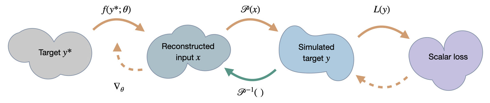
Fig. 51 A visual overview of the different spaces involved in SIP training.#
To join these three pieces together, we use the following algorithm. As introduced by Holl et al. [HKT22], we’ll denote this training process as scale-invariant physics (SIP) training.
Scale-Invariant Physics (SIP) Training
To update the weights \(\theta\) of the NN \(f\), we perform the following update step:
Given a set of inputs \(y^*\), evaluate the forward pass to compute the NN prediction \(x = f(y^*; \theta)\)
Compute \(y\) via a forward simulation (\(y = \mathcal P(x)\)) and invoke the (local) inverse simulator \(P^{-1}(y; x)\) to obtain the step \(\Delta x_{\text{PG}} = \mathcal P^{-1} (y + \eta \Delta y; x)\) with \(\Delta y = y^* - y\)
Evaluate the network loss, e.g., \(L = \frac 1 2 | x - \tilde x |_2^2\) with \(\tilde x = x+\Delta x_{\text{PG}}\), and perform a Newton step treating \(\tilde x\) as a constant
Use GD (or a GD-based optimizer like Adam) to propagate the change in \(x\) to the network weights \(\theta\) with a learning rate \(\eta_{\text{NN}}\)
This combined optimization algorithm depends on both the learning rate \(\eta_\textrm{NN}\) for the network as well as the step size \(\eta\) from above, which factors into \(\Delta y\). To first order, the effective learning rate of the network weights is \(\eta_\textrm{eff} = \eta \cdot \eta_\textrm{NN}\). We recommend setting \(\eta\) as large as the accuracy of the inverse simulator allows. In many cases \(\eta=1\) is possible, otherwise \(\eta_\textrm{NN}\) should be adjusted accordingly. This allows for nonlinearities of the simulator to be maximally helpful in adjusting the optimization direction.
This algorithm combines the inverse simulator to compute accurate, higher-order updates with traditional training schemes for NN representations. This is an attractive property, as we have a large collection of powerful methodologies for training NNs that stay relevant in this way. The treatment of the loss functions as “glue” between NN and physics component plays a central role here.

Loss functions#
In the above algorithm, we have assumed an \(L^2\) loss, and without further explanation introduced a Newton step to propagate the inverse simulator step to the NN. Below, we explain and justify this treatment in more detail.
The central reason for introducing a Newton step is the improved accuracy for the loss derivative. Unlike with regular Newton or the quasi-Newton methods from equation (34), we do not need the Hessian of the full system. Instead, the Hessian is only needed for \(L(y)\). This makes Newton’s method attractive again. Even better, for many typical \(L\) the analytical form of the Newton updates is known.
E.g., consider the most common supervised objective function, \(L(y) = \frac 1 2 | y - y^*|_2^2\) as already put to use above. \(y\) denotes the predicted, and \(y^*\) the target value. We then have \(\frac{\partial L}{\partial y} = y - y^*\) and \(\frac{\partial^2 L}{\partial y^2} = 1\). Using equation (34), we get \(\Delta y = \eta \cdot (y^* - y)\) which can be computed right away, without evaluating any additional Hessian matrices.
Once \(\Delta y\) is determined, the gradient can be backpropagated to \(x\), e.g. an earlier time, using the inverse simulator \(\mathcal P^{-1}\). We’ve already used this combination of a Newton step for the loss and an inverse simulator for the PDE in Simple Example comparing Different Optimizers.
The loss in \(x\) here acts as a proxy to embed the update from the inverse simulator into the network training pipeline. It is not to be confused with a traditional supervised loss in \(x\) space. Due to the dependency of \(\mathcal P^{-1}\) on the prediction \(y\), it does not average multiple modes of solutions in \(x\). To demonstrate this, consider the case that GD is being used as solver for the inverse simulation. Then the total loss is purely defined in \(y\) space, reducing to a regular first-order optimization.
Hence, to summarize with SIPs we employ a trivial Newton step for the loss in \(y\), and a proxy \(L^2\) loss in \(x\) that connects the computational graphs of inverse physics and NN for backpropagation. The following figure visualizes the different steps.
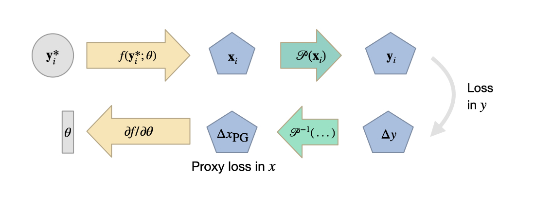
Fig. 52 A visual overview of SIP training for an entry \(i\) of a mini-batch, including the two loss computations in \(y\) and in \(x\) space (for the proxy loss).#
Iterations and time dependence#
The above procedure describes the optimization of neural networks that make a single prediction. This is suitable for scenarios to reconstruct the state of a system at \(t_0\) given the state at a \(t_e > t_0\) or to estimate an optimal initial state to match certain conditions at \(t_e\).
However, the SIP method can also be applied to more complex setups involving multiple objectives and multiple network interactions at different times. Such scenarios arise e.g. in control tasks, where a network induces small forces at every time step to reach a certain physical state at \(t_e\). It also occurs in correction tasks where a network tries to improve the simulation quality by performing corrections at every time step.
In these scenarios, the process above (Newton step for loss, inverse simulator step for physics, GD for the NN) is iteratively repeated, e.g., over the course of different time steps, leading to a series of additive terms in \(L\). This typically makes the learning task more difficult, as we repeatedly backpropagate through the iterations of the physical solver and the NN, but the SIP algorithm above extends to these case just like a regular GD training.
SIP training in action#
Let’s illustrate the convergence behavior of SIP training and how it depends on characteristics of \(\mathcal P\) with an example [HKT22]. We consider the synthetic two-dimensional function
where \(R_\phi \in \mathrm{SO}(2)\) denotes a rotation matrix. The parameters \(\xi\) and \(\phi\) allow us to continuously change the characteristics of the system. The value of \(\xi\) determines the conditioning of \(\mathcal P\) with large \(\xi\) representing ill-conditioned problems while \(\phi\) describes the coupling of \(x_1\) and \(x_2\). When \(\phi=0\), the off-diagonal elements of the Hessian vanish and the problem factors into two independent problems.
Here’s an example of the resulting loss landscape for \(y^*=(0.3, -0.5)\), \(\xi=1\), \(\phi=15^\circ\) that shows the entangling of the sine function for \(x_1\) and linear change for \(x_2\):

Next we train a fully-connected neural network to invert this problem via equation (37). We’ll compare SIP training using a saddle-free Newton solver to various state-of-the-art network optimizers. For fairness, the best learning rate is selected independently for each optimizer. When choosing \(\xi=1\) the problem is perfectly conditioned. In this case all network optimizers converge, with Adam having a slight advantage. This is shown in the left graph:

Fig. 53 Loss over time in seconds for a well-conditioned (left), and ill-conditioned case (right).#
At \(\xi=32\), we have a fairly badly conditioned case, and only SIP and Adam succeed in optimizing the network to a significant degree, as shown on the right.
Note that the two graphs above show convergence over time. The relatively slow convergence of SIP mostly stems from it taking significantly more time per iteration than the other methods, on average 3 times as long as Adam. While the evaluation of the Hessian inherently requires more computations, the per-iteration time of SIP could likely be significantly reduced by optimizing the computations.
By increasing \(\xi\) while keeping \(\phi=0\) fixed we can show how the conditioning continually influences the different methods, as shown on the left here:

Fig. 54 Performance when varying the conditiong (left) and the entangling of dimensions via the rotation (right).#
The accuracy of all traditional network optimizers decreases because the gradients scale with \((1/\xi, \xi)\) in \(x\), becoming longer in \(x_2\), the direction that requires more precise values. SIP training avoids this using the Hessian, inverting the scaling behavior and producing updates that align with the flat direction in \(x\). This allows SIP training to retain its relative accuracy over a wide range of \(\xi\). Even for Adam, the accuracy becomes worse for larger \(\xi\).
By varying only \(\phi\) we can demonstrate how the entangling of the different components influences the behavior of the optimizers. The right graph of Fig. 54 varies \(\phi\) with \(\xi=32\) fixed. This sheds light on how Adam manages to learn in ill-conditioned settings. Its diagonal approximation of the Hessian reduces the scaling effect when \(x_1\) and \(x_2\) lie on different scales, but when the parameters are coupled, the lack of off-diagonal terms prevents this. It’s performance deteriorates by more than an order of magnitude in this case. SIP training has no problem with coupled parameters since its update steps for the optimization are using the full-rank Hessian \(\frac{\partial^2 L}{\partial x}\). Thus, the SIP training yields the best results across the varying optimization problems posed by this example setup.

Discussion of SIP Training#
Although we’ve only looked at smaller toy problems so far, we’ll pull the discussion of SIP training forward. The next chapter will illustrate this with a more complex example, but as we’ll directly switch to a new algorithm afterwards, below is a better place for a discussion of the properties of SIP.
Overall, the scale-invariance of SIP training allows it to find solutions exponentially faster than other learning methods for many physics problems, while keeping the computational cost relatively low. It provably converges when enough network updates \(\Delta\theta\) are performed per solver evaluation and it can be shown that it converges with a single \(\Delta\theta\) update for a wide range of physics experiments.
Limitations#
While SIP training can find vastly more accurate solutions, there are some caveats to consider.
First, an approximately scale-invariant physics solver is required. While in low-dimensional \(x\) spaces, Newton’s method is a good candidate, high-dimensional spaces require some other form of inversion. Some equations can locally be inverted analytically but for complex problems, domain-specific knowledge may be required, or we can employ to numerical methods (coming up).
Second, SIP focuses on an accurate inversion of the physics part, but uses traditional first-order optimizers to determine \(\Delta\theta\). As discussed, these solvers behave poorly in ill-conditioned settings which can also affect SIP performance when the network outputs lie on very different scales. Thus, we should keep inversion for the NN in mind as a goal.
Third, while SIP training generally leads to more accurate solutions, measured in \(x\) space, the same is not always true for the loss \(L = \sum_i L_i\). SIP training weighs all examples equally, independent of their loss values. This can be useful, but it can cause problems in examples where regions with overly small or large curvatures \(|\frac{\partial^2L}{\partial x^2}|\) distort the importance of samples. In these cases, or when the accuracy in \(x\) space is not important, like in control tasks, traditional training methods may perform better than SIP training.
Similarities to supervised training#
Interestingly, the SIP training resembles the supervised approaches from Supervised Training. It effectively yields a method that provides reliable updates which are computed on-the-fly, at training time. The inverse simulator provides the desired inversion, possibly with a high-order method, and avoids the averaging of multi modal solutions (cf. A Teaser Example).
The latter is one of the main advantages of this setup: a pre-computed data set can not take multi-modality into account, and hence inevitably leads to suboptimal solutions being learned once the mapping from input to reference solutions is not unique.
At the same time this illustrates a difficulty of the DP training from Introduction to Differentiable Physics: the gradients it yields are not properly inverted, and are difficult to reliably normalize via pre-processing. Hence they can lead to the scaling problems discussing in Scale-Invariance and Inversion, and correspondingly give vanishing and exploding gradients at training time. These problems are what we’re targeting in this chapter.
In the next section we’ll show a more complex example of training physics-based NNs with SIP updates from inverse simulators, before explaining a second alternative for tackling the scaling problems.