Introduction to Differentiable Physics#
As a next step towards a tighter and more generic combination of deep learning methods and physical simulations we will target incorporating differentiable numerical simulations into the learning process. In the following, we’ll shorten these “differentiable numerical simulations of physical systems” to just “differentiable physics” (DP).
The central goal of these methods is to use existing numerical solvers to empower and improve AI systems. This requires equipping them with functionality to compute gradients with respect to their inputs. Once this is realized for all operators of a simulation, we can leverage the autodiff functionality of DL frameworks with backpropagation to let gradient information flow from a simulator into an NN and vice versa. This has numerous advantages such as improved learning feedback and generalization, as we’ll outline below.
In contrast to the physics-informed loss functions of the previous chapter, it also enables handling more complex solution manifolds instead of single inverse problems. E.g., instead of using deep learning to solve single inverse problems as in the previous chapter, differentiable physics can be used to train NNs that learn to solve larger classes of inverse problems very efficiently.
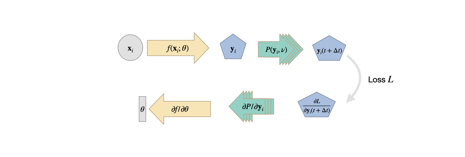
Fig. 15 Training with differentiable physics means that a chain of differentiable operators provide directions in the form of gradients to steer the learning process.#
Differentiable operators#
With DP we build on existing numerical solvers. I.e., the approach is strongly relying on the algorithms developed in the larger field of computational methods for a vast range of physical effects in our world. To start with, we need a continuous formulation as model for the physical effect that we’d like to simulate – if this is missing we’re in trouble. But luckily, we can tap into existing collections of model equations and established methods for discretizing continuous models.
Let’s assume we have a continuous formulation \(\mathcal P^*(\mathbf{u}, \nu)\) of the physical quantity of interest \(\mathbf{u}(\mathbf{u}, t): \mathbb R^d \times \mathbb R^+ \rightarrow \mathbb R^d\), with model parameters \(\nu\) (e.g., diffusion, viscosity, or conductivity constants). The components of \(\mathbf{u}\) will be denoted by a numbered subscript, i.e., \(\mathbf{u} = (u_1,u_2,\dots,u_d)^T\). Typically, we are interested in the temporal evolution of such a system. Discretization yields a formulation \(\mathcal P(\mathbf{u}, \nu)\) that we re-arrange to compute a future state after a time step \(\Delta t\). The state at \(t+\Delta t\) is computed via sequence of operations \(\mathcal P_1, \mathcal P_2 \dots \mathcal P_m\) such that \(\mathbf{u}(t+\Delta t) = \mathcal P_m \circ \dots \mathcal P_2 \circ \mathcal P_1 ( \mathbf{u}(t),\nu )\), where \(\circ\) denotes function decomposition, i.e. \(f(g(x)) = f \circ g(x)\).
Note
In order to integrate this solver into a DL process, we need to ensure that every operator \(\mathcal P_i\) provides a gradient w.r.t. its inputs, i.e. in the example above \(\partial \mathcal P_i / \partial \mathbf{u}\).
Note that we typically don’t need derivatives for all parameters of \(\mathcal P(\mathbf{u}, \nu)\), e.g., we omit \(\nu\) in the following, assuming that this is a given model parameter with which the NN should not interact. Naturally, it can vary within the solution manifold that we’re interested in, but \(\nu\) will not be the output of an NN representation. If this is the case, we can omit providing \(\partial \mathcal P_i / \partial \nu\) in our solver. However, the following learning process naturally transfers to including \(\nu\) as a degree of freedom.
Jacobians#
As \(\mathbf{u}\) is typically a vector-valued function, \(\partial \mathcal P_i / \partial \mathbf{u}\) denotes a Jacobian matrix \(J\) rather than a single value:
where, as above, \(d\) denotes the number of components in \(\mathbf{u}\). As \(\mathcal P\) maps one value of \(\mathbf{u}\) to another, the Jacobian is square here. Of course this isn’t necessarily the case for general model equations, but non-square Jacobian matrices would not cause any problems for differentiable simulations.
In practice, we rely on the reverse mode differentiation that all modern DL frameworks provide, and focus on computing a matrix vector product of the Jacobian transpose with a vector \(\mathbf{a}\), i.e. the expression: \( \big( \frac{\partial \mathcal P_i }{ \partial \mathbf{u} } \big)^T \mathbf{a} \). If we’d need to construct and store all full Jacobian matrices that we encounter during training, this would cause huge memory overheads and unnecessarily slow down training. Instead, for backpropagation, we can provide faster operations that compute products with the Jacobian transpose because we always have a scalar loss function at the end of the chain.
Given the formulation above, we need to resolve the derivatives of the chain of function compositions of the \(\mathcal P_i\) at some current state \(\mathbf{u}^n\) via the chain rule. E.g., for two of them
which is just the vector valued version of the “classic” chain rule \(f\big(g(x)\big)' = f'\big(g(x)\big) g'(x)\), and directly extends for larger numbers of composited functions, i.e. \(i>2\).
Here, the derivatives for \(\mathcal P_1\) and \(\mathcal P_2\) are still Jacobian matrices, but knowing that at the “end” of the chain we have our scalar loss (cf. Overview), the right-most Jacobian will invariably be a matrix with 1 column, i.e. a vector. During reverse mode, we start with this vector, and compute the multiplications with the left Jacobians, \(\frac{ \partial \mathcal P_1 }{ \partial \mathbf{u} }\) above, one by one.
For the details of forward and reverse mode differentiation, please check out external materials such as this nice survey by Baydin et al..
Learning via DP operators#
Thus, once the operators of our simulator support computations of the Jacobian-vector products, we can integrate them into DL pipelines just like you would include a regular fully-connected layer or a ReLU activation.
At this point, the following (very valid) question arises: “Most physics solvers can be broken down into a sequence of vector and matrix operations. All state-of-the-art DL frameworks support these, so why don’t we just use these operators to realize our physics solver?”
It’s true that this would theoretically be possible. The problem here is that each of the vector and matrix operations in tensorflow and pytorch is computed individually, and internally needs to store the current state of the forward evaluation for backpropagation (the “\(g(x)\)” above). For a typical simulation, however, we’re not overly interested in every single intermediate result our solver produces. Typically, we’re more concerned with significant updates such as the step from \(\mathbf{u}(t)\) to \(\mathbf{u}(t+\Delta t)\).
Thus, in practice it is a very good idea to break down the solving process into a sequence of meaningful but monolithic operators. This not only saves a lot of work by preventing the calculation of unnecessary intermediate results, it also allows us to choose the best possible numerical methods to compute the updates (and derivatives) for these operators. E.g., as this process is very similar to adjoint method optimizations, we can re-use many of the techniques that were developed in this field, or leverage established numerical methods. E.g., we could leverage the \(O(n)\) runtime of multigrid solvers for matrix inversion.
The flip-side of this approach is that it requires some understanding of the problem at hand, and of the numerical methods. Also, a given solver might not provide gradient calculations out of the box. Thus, if we want to employ DL for model equations that we don’t have a proper grasp of, it might not be a good idea to directly go for learning via a DP approach. However, if we don’t really understand our model, we probably should go back to studying it a bit more anyway…
Also, in practice we should be greedy with the derivative operators, and only provide those which are relevant for the learning task. E.g., if our network never produces the parameter \(\nu\) in the example above, and it doesn’t appear in our loss formulation, we will never encounter a \(\partial/\partial \nu\) derivative in our backpropagation step.
The following figure summarizes the DP-based learning approach, and illustrates the sequence of operations that are typically processed within a single PDE solve. As many of the operations are non-linear in practice, this often leads to a challenging learning task for the NN:
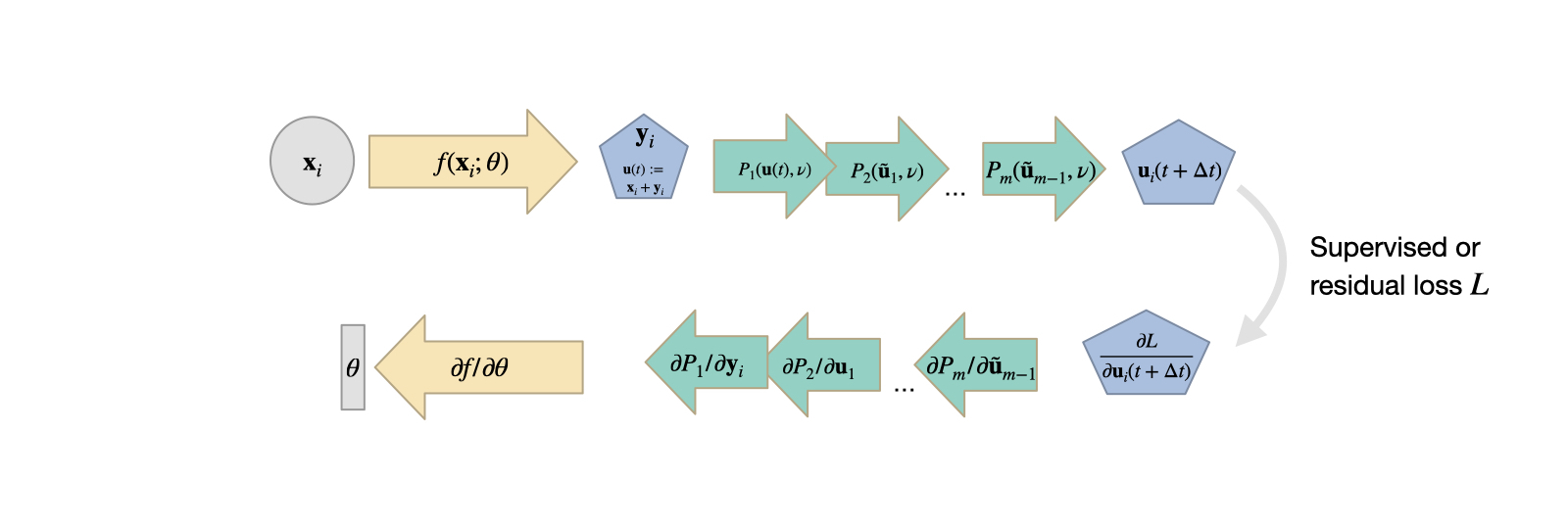
Fig. 16 DP learning with a PDE solver that consists of \(m\) individual operators \(\mathcal P_i\). The gradient travels backward through all \(m\) operators before influencing the network weights \(\theta\).#
A practical example#
As a simple example let’s consider the advection of a passive scalar density \(d(\mathbf{x},t)\) in a velocity field \(\mathbf{u}\) as physical model \(\mathcal P^*\):
Instead of using this formulation as a residual equation right away (as in v2 of Physical Loss Terms), we can discretize it with our favorite mesh and discretization scheme, to obtain a formulation that updates the state of our system over time. This is a standard procedure for a forward solve. To simplify things, we assume here that \(\mathbf{u}\) is only a function in space, i.e. constant over time. We’ll bring back the time evolution of \(\mathbf{u}\) later on.
Let’s denote this re-formulation as \(\mathcal P\). It maps a state of \(d(t)\) into a new state at an evolved time, i.e.:
As a simple example of an inverse problem and learning task, let’s consider the problem of finding a velocity field \(\mathbf{u}\). This velocity should transform a given initial scalar density state \(d^{~0}\) at time \(t^0\) into a state that’s evolved by \(\mathcal P\) to a later “end” time \(t^e\) with a certain shape or configuration \(d^{\text{target}}\). Informally, we’d like to find a flow that deforms \(d^{~0}\) through the PDE model into a target state. The simplest way to express this goal is via an \(L^2\) loss between the two states. So we want to minimize the loss function \(L=|d(t^e) - d^{\text{target}}|^2\).
Note that as described here, this inverse problem is a pure optimization task: there’s no NN involved, and our goal is to obtain \(\mathbf{u}\). We do not want to apply this velocity to other, unseen test data, as would be custom in a real learning task.
The final state of our marker density \(d(t^e)\) is fully determined by the evolution from \(\mathcal P\) via \(\mathbf{u}\), which gives the following minimization problem:
We’d now like to find the minimizer for this objective by gradient descent (GD), where the gradient is determined by the differentiable physics approach described earlier in this chapter. Once things are working with GD, we can relatively easily switch to better optimizers or bring an NN into the picture, hence it’s always a good starting point. To make things easier to read below, we’ll omit the transpose of the Jacobians in the following. Unfortunately, the Jacobian is defined this way, but we actually never need the un-transposed one. Keep in mind that in practice we’re dealing with transposed Jacobians \(\big( \frac{ \partial a }{ \partial b} \big)^T\) that are “abbreviated” by \(\frac{ \partial a }{ \partial b}\).
As the discretized velocity field \(\mathbf{u}\) contains all our degrees of freedom, all we need to do is to update the velocity by an amount \(\Delta \mathbf{u} = \partial L / \partial \mathbf{u}\), which is decomposed into \(\Delta \mathbf{u} = \frac{ \partial d }{ \partial \mathbf{u}} \frac{ \partial L }{ \partial d} \).
The \(\frac{ \partial L }{ \partial d}\) component is typically simple enough: we’ll get
If \(d\) is represented as a vector, e.g., for one entry per cell of a mesh, \(\frac{ \partial L }{ \partial d}\) will likewise be a column vector of equivalent size. This stems from the fact that \(L\) is always a scalar loss function, and so the Jacobian matrix will have a dimension of 1 along the \(L\) dimension. Intuitively, this vector will simply contain the differences between \(d\) at the end time in comparison to the target densities \(d^{\text{target}}\).
The evolution of \(d\) itself is given by our discretized physical model \(\mathcal P\), and we use \(\mathcal P\) and \(d\) interchangeably. Hence, the more interesting component is the Jacobian \(\partial d / \partial \mathbf{u} = \partial \mathcal P / \partial \mathbf{u}\) to compute the full \(\Delta \mathbf{u} = \frac{ \partial d }{ \partial \mathbf{u}} \frac{ \partial L }{ \partial d}\). We luckily don’t need \(\partial d / \partial \mathbf{u}\) as a full matrix, but instead only multiplied by \(\frac{ \partial L }{ \partial d}\).
So what is the actual Jacobian for \(d\)? To compute it we first need to finalize our PDE model \(\mathcal P\), such that we get an expression which we can derive. In the next section we’ll choose a specific advection scheme and a discretization so that we can be more specific.
Introducing a specific advection scheme#
In the following we’ll make use of a simple first order upwinding scheme on a Cartesian grid in 1D, with marker density \(d_i\) and velocity \(u_i\) for cell \(i\). We omit the \((t)\) for quantities at time \(t\) for brevity, i.e., \(d_i(t)\) is written as \(d_i\) below. From above, we’ll use our physical model that updates the marker density \(d_i(t+\Delta t) = \mathcal P ( d_i(t), \mathbf{u}(t), t + \Delta t)\), which gives the following:
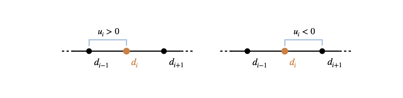
Fig. 17 1st-order upwinding uses a simple one-sided finite-difference stencil that takes into account the direction of the flow#
Thus, for a negative \(u_i\), we’re using \(u_i^+\) to look in the opposite direction of the velocity, i.e., backward in terms of the motion. \(u_i^-\) will be zero in this case. For positive \(u_i\) it’s vice versa, and we’ll get a zero’ed \(u_i^+\), and a backward difference stencil via \(u_i^-\). To pick the former case, for a negative \(u_i\) we get
and hence \(\partial \mathcal P / \partial u_i\) gives \(\frac{\Delta t }{ \Delta x} d_i - \frac{\Delta t }{ \Delta x} d_{i+1}\). Intuitively, the change of the velocity \(u_i\) depends on the spatial derivatives of the densities. Due to the first order upwinding, we only include two neighbors (higher order methods would depend on additional entries of \(d\))
In practice this step is equivalent to evaluating a transposed matrix multiplication. If we rewrite the calculation above as \( \mathcal P ( d_i(t), \mathbf{u}(t), t + \Delta t) = A \mathbf{u}\), then \(\big( \partial \mathcal P / \partial \mathbf{u} \big)^T = A^T\). However, in many practical cases, a matrix free implementation of this multiplication might be preferable to actually constructing \(A\).
Another derivative that we can consider for the advection scheme is that w.r.t. the previous density state, i.e. \(d_i(t)\), which is \(d_i\) in the shortened notation. \(\partial \mathcal P / \partial d_i\) for cell \(i\) from above gives \(1 + \frac{u_i \Delta t }{ \Delta x}\). However, for the full gradient we’d need to add the potential contributions from cells \(i+1\) and \(i-1\), depending on the sign of their velocities. This derivative will come into play in the next section.
Time evolution#
So far we’ve only dealt with a single update step of \(d\) from time \(t\) to \(t+\Delta t\), but we could of course have an arbitrary number of such steps. After all, above we stated the goal to advance the initial marker state \(d(t^0)\) to the target state at time \(t^e\), which could encompass a long interval of time.
In the expression above for \(d_i(t+\Delta t)\), each of the \(d_i(t)\) in turn depends on the velocity and density states at time \(t-\Delta t\), i.e., \(d_i(t-\Delta t)\). Thus we have to trace back the influence of our loss \(L\) all the way back to how \(\mathbf{u}\) influences the initial marker state. This can involve a large number of evaluations of our advection scheme via \(\mathcal P\).
This sounds challenging at first: e.g., one could try to insert equation (17) at time \(t-\Delta t\) into equation (17) at time \(t\) and repeat this process recursively until we have a single expression relating \(d^{~0}\) to the targets. However, thanks to the linear nature of the Jacobians, we treat each advection step, i.e., each invocation of our PDE \(\mathcal P\) as a separate, modular operation. And each of these invocations follows the procedure described in the previous section.
Given the machinery above, the backtrace is fairly simple to realize: for each of the advection steps in \(\mathcal P\) we compute a Jacobian product with the incoming vector of derivatives from the loss \(L\) or a previous advection step. We repeat this until we have traced the chain from the loss with \(d^{\text{target}}\) all the way back to \(d^{~0}\). Theoretically, the velocity \(\mathbf{u}\) could be a function of time like \(d\), in which case we’d get a gradient \(\Delta \mathbf{u}(t)\) for every time step \(t\). However, to simplify things below, let’s we assume we have field that is constant in time, i.e., we’re reusing the same velocities \(\mathbf{u}\) for every advection via \(\mathcal P\). Now, each time step will give us a contribution to \(\Delta \mathbf{u}\) which we accumulate for all steps.
Here the last term above contains the full backtrace of the marker density to time \(t^0\). The terms of this sum look unwieldy at first, but looking closely, each line simply adds an additional Jacobian for one time step on the left hand side. This follows from the chain rule, as shown in the two-operator case above. So the terms of the sum contain a lot of similar Jacobians, and in practice can be computed efficiently by backtracing through the sequence of computational steps that resulted from the forward evaluation of our PDE. (Note that, as mentioned above, we’ve omitted the transpose of the Jacobians here.)
This structure also makes clear that the process is very similar to the regular training process of an NN: the evaluations of these Jacobian vector products from nested function calls is exactly what a deep learning framework does for training an NN (we just have weights \(\theta\) instead of a velocity field there). And hence all we need to do in practice is to provide a custom function the Jacobian vector product for \(\mathcal P\).
Implicit gradient calculations#
As a slightly more complex example let’s consider Poisson’s equation \(\nabla^2 a = b\), where \(a\) is the quantity of interest, and \(b\) is given. This is a very fundamental elliptic PDE that is important for a variety of physical problems, from electrostatics to gravitational fields. It also arises in the context of fluids, where \(a\) takes the role of a scalar pressure field in the fluid, and the right hand side \(b\) is given by the divergence of the fluid velocity \(\mathbf{u}\).
For fluids, we typically have \(\mathbf{u}^{n} = \mathbf{u} - \nabla p\), with \(\nabla^2 p = \nabla \cdot \mathbf{u}\). Here, \(\mathbf{u}^{n}\) denotes the new, divergence-free velocity field. This step is typically crucial to enforce the hard-constraint \(\nabla \cdot \mathbf{u}=0\), and also goes under the name of Chorin Projection, or Helmholtz decomposition. It is a direct consequence of the fundamental theorem of vector calculus.
If we now introduce an NN that modifies \(\mathbf{u}\) in a solver, we inevitably have to backpropagate through the Poisson solve. I.e., we need a gradient for \(\mathbf{u}^{n}\), which in this notation takes the form \(\partial \mathbf{u}^{n} / \partial \mathbf{u}\).
In combination, we aim for computing \(\mathbf{u}^{n} = \mathbf{u} - \nabla \left( (\nabla^2)^{-1} \nabla \cdot \mathbf{u} \right)\). The outer gradient (from \(\nabla p\)) and the inner divergence (\(\nabla \cdot \mathbf{u}\)) are both linear operators, and their gradients are simple to compute. The main difficulty lies in obtaining the matrix inverse \((\nabla^2)^{-1}\) from Poisson’s equation (we’ll keep it a bit simpler here, but it’s often time-dependent, and non-linear).
In practice, the matrix vector product for \((\nabla^2)^{-1} b\) with \(b=\nabla \cdot \mathbf{u}\) is not explicitly computed via matrix operations, but approximated with a (potentially matrix-free) iterative solver. E.g., conjugate gradient (CG) methods are a very popular choice here. Thus, we theoretically could treat this iterative solver as a function \(\mathcal{S}\), with \(p = \mathcal{S}(\nabla \cdot \mathbf{u})\). It’s worth noting that matrix inversion is a non-linear process, despite the matrix itself being linear. As solvers like CG are also based on matrix and vector operations, we could decompose \(\mathcal{S}\) into a sequence of simpler operations over the course of all solver iterations as \(\mathcal{S}(x) = \mathcal{S}_n( \mathcal{S}_{n-1}(...\mathcal{S}_{1}(x)))\), and backpropagate through each of them. This is certainly possible, but not a good idea: it can introduce numerical problems, and will be very slow. As mentioned above, by default DL frameworks store the internal states for every differentiable operator like the \(\mathcal{S}_i()\) in this example, and hence we’d organize and keep a potentially huge number of intermediate states in memory. These states are completely uninteresting for our original PDE, though. They’re just intermediate states of the CG solver.
If we take a step back and look at \(p = (\nabla^2)^{-1} b\), it’s gradient \(\partial p / \partial b\) is just \(((\nabla^2)^{-1})^T\). And in this case, \((\nabla^2)\) is a symmetric matrix, and so \(((\nabla^2)^{-1})^T=(\nabla^2)^{-1}\). This is the identical inverse matrix that we encountered in the original equation above, and hence we re-use our unmodified iterative solver to compute the gradient. We don’t need to take it apart and slow it down by storing intermediate states. However, the iterative solver computes the matrix-vector-products for \((\nabla^2)^{-1} b\). So what is \(b\) during backpropagation? In an optimization setting we’ll always have our loss function \(L\) at the end of the forward chain. The backpropagation step will then give a gradient for the output, let’s assume it is \(\partial L/\partial p\) here, which needs to be propagated to the earlier operations of the forward pass. Thus, we simply invoke our iterative solve during the backward pass to compute \(\partial p / \partial b = \mathcal{S}(\partial L/\partial p)\). And assuming that we’ve chosen a good solver as \(\mathcal{S}\) for the forward pass, we get exactly the same performance and accuracy in the backwards pass.
If you’re interested in a code example, the differentiate-pressure example of phiflow uses exactly this process for an optimization through a pressure projection step: a flow field that is constrained on the right side, is optimized for the content on the left, such that it matches the target on the right after a pressure projection step.
The main take-away here is: it is important not to blindly backpropagate through the forward computation, but to think about which steps of the analytic equations for the forward pass to compute gradients for. In cases like the above, we can often find improved analytic expressions for the gradients, which we then approximate numerically.
Implicit Function Theorem & Time
IFT: The process above essentially yields an implicit derivative. Instead of explicitly deriving all forward steps, we’ve relied on the implicit function theorem to compute the derivative.
Time: we can actually consider the steps of an iterative solver as a virtual “time”, and backpropagate through these steps. In line with other DP approaches, this enables an NN to interact with an iterative solver. An example is to learn initial guesses of CG solvers from [UBH+20]. Details and code can be found here.
Summary of differentiable physics so far#
To summarize, using differentiable physical simulations gives us a tool to include physical equations with a chosen discretization into DL. In contrast to the residual constraints of the previous chapter, this makes it possible to let NNs seamlessly interact with physical solvers.
We’d previously fully discard our physical model and solver once the NN is trained: in the example from Burgers Optimization with a PINN the NN gives us the solution directly, bypassing any solver or model equation. The DP approach substantially differs from the physics-informed NNs (v2) from Physical Loss Terms, it has more in common with the controlled discretizations (v1). They are essentially a subset, or partial application of DP training.
However in contrast to both residual approaches, DP makes it possible to train an NN alongside a numerical solver, and thus we can make use of the physical model (as represented by the solver) later on at inference time. This allows us to move beyond solving single inverse problems, and yields NNs that quite robustly generalize to new inputs. Let’s revisit the example problem from Burgers Optimization with a PINN in the context of DPs.