A Teaser Example

Let’s start with a very reduced example that highlights some of the key capabilities of physics-based learning approaches. Let’s assume our physical model is a very simple equation: a parabola along the positive x-axis. We’ll also directly use this example to give an outlook towards probabilistic “generative AI” approaches.

Despite being very simple, there are two solutions for every point along x, i.e. we have two modes, one above the other one below the x-axis, as shown on the left below. If we don’t take care, a conventional learning approach will give us an approximation like the red one shown in the middle, which is completely off. With an improved learning setup, e.g., by using a discretized numerical solver, we can at least accurately represent one of the modes of the solution (shown in green on the right). Interestingly, approaches that learn the full distribution at each point, flow matching as a representative of diffusion models is used below, can capture both modes!

Fig. 2 Side by side - supervised versus differentiable physics and probabilistic training.

Differentiable physics

One of the key concepts of the following chapters is what we’ll call differentiable physics (DP). This means that we use domain knowledge in the form of model equations, and then integrate discretized versions of these models into the training process. As implied by the name, having differentiable formulations and operators is crucial for this process to integrate with neural networks training.

Let’s illustrate the properties of deep learning via DP with the following example: We’d like to find an unknown function \(f^*\) that generates solutions from a space \(Y\), taking inputs from \(X\), i.e. \(f^*: X \to Y\). In the following, we’ll often denote idealized, and unknown functions with a \(*\) superscript, in contrast to their discretized, realizable counterparts without this superscript. Let’s additionally assume we have a generic differential equation \(\mathcal P^*: Y \to Z\) (our model equation), that encodes a property of the solutions, e.g. some real world behavior we’d like to match. Later on, \(P^*\) will often represent time evolutions, but it could also be a conservation law (e.g., conservation of mass, then \(\mathcal P^*\) would measure divergence).

Using a neural network \(f\) to learn the unknown and ideal function \(f^*\), we could turn to classic supervised training to obtain \(f\) by collecting data. This classical setup requires a dataset by sampling \(x\) from \(X\) and adding the corresponding solutions \(y\) from \(Y\). We could obtain these, e.g., by classical numerical techniques. Then we train the NN \(f\) with classic methods using this dataset.

In contrast to this supervised approach, employing a differentiable physics approach takes advantage of the fact that we can often use a discretized version of the physical model \(\mathcal P\) and employ it to guide the training of \(f\). I.e., we want \(f\) to be aware of our simulator \(\mathcal P\), and to interact with it. This can give fundamental improvements, as we’ll illustrate below with a very simple example (more complex ones will follow later on).

Note that in order for the DP approach to work, \(\mathcal P\) has to be differentiable, as implied by the name. These differentials, in the form of a gradient, are what’s driving the learning process and neural network integration.

Finding the inverse function of a parabola

To illustrate the difference of supervised and DP approaches, we consider the following simplified setting: Given the function \(\mathcal P: y\to y^2\) for \(y\) in the interval \([0,1]\), find the unknown function \(f\) such that \(\mathcal P(f(x)) = x\) for all \(x\) in \([0,1]\). E.g., for \(x=0.5\), solutions would be \(\pm\sqrt{0.5}\). Note: to make things a bit more interesting, we’re using \(y^2\) here for \(\mathcal P\) instead of the more common \(x^2\) parabola, and the discretization is simply given by representing the \(x\) and \(y\) via floating point numbers in the computer for this simple case.

We know that possible solutions for \(f\) are the positive or negative square root function (for completeness: piecewise combinations would also be possible). This sounds easy, so let’s try to train a neural network to approximate this inverse mapping \(f\). Doing this in the “classical” supervised manner, i.e. purely based on data, is an obvious starting point. After all, this approach was shown to be a powerful tool for a variety of other applications, e.g., in computer vision.

import numpy as np
import torch
import torch.nn as nn
import torch.optim as optim

For supervised training, we can employ our solver \(\mathcal P\) for the problem to pre-compute the solutions we need for training: We randomly choose between the positive and the negative square root. This resembles the general case, where we would gather all data beforehand, e.g., using optimization techniques to compute the solutions or even experiments. This data collection typically does not favor one particular mode from multimodal solutions.

# Generate data
N = 10000
X = np.random.random(N).astype(np.float32).reshape(-1, 1)

# Generation of Y-Data
sign = (- np.ones((N,))).astype(np.float32) ** np.random.randint(2, size=N)
Y = (np.sqrt(X.flatten()) * sign).reshape(-1, 1).astype(np.float32)

# Convert to PyTorch tensors
X_tensor = torch.tensor(X)
Y_tensor = torch.tensor(Y)

Now we can define a network. We’ll use a simple fully connected architecture with three hidden layers and ReLU activations.

# Define the neural network
class SimpleNN(nn.Module):
    def __init__(self, hiddendim=10):
        super(SimpleNN, self).__init__()
        self.fc1 = nn.Linear(1, hiddendim)
        self.fc2 = nn.Linear(hiddendim, hiddendim)
        self.fc3 = nn.Linear(hiddendim, 1)
        self.relu = nn.ReLU()
    
    def forward(self, x):
        x = self.relu(self.fc1(x))
        x = self.relu(self.fc2(x))
        x = self.fc3(x)  # Linear output
        return x

Next we can instantiate the model (using a hidden dimension of 128), specify a loss function (will used a simple mean squared error with PyTorch’s MSELoss()), and the Adam optimizer. The network is trained for 50 epochs in the loop below:

nn_sup = SimpleNN(hiddendim=128)
criterion = nn.MSELoss()
optimizer = optim.Adam(nn_sup.parameters(), lr=0.001)

# Training loop
epochs = 50
batch_size = 5

for epoch in range(epochs):
    permutation = torch.randperm(N)
    epoch_loss = 0.0
    
    for i in range(0, N, batch_size):
        indices = permutation[i:i+batch_size]
        batch_x, batch_y = X_tensor[indices], Y_tensor[indices]
        
        optimizer.zero_grad()
        outputs = nn_sup(batch_x)
        loss = criterion(outputs, batch_y)
        loss.backward()
        optimizer.step()
        
        epoch_loss += loss.item()
    
    if(epoch%10==9): print(f"Epoch {epoch+1}/{epochs}, Loss: {epoch_loss/N:.6f}")

Epoch 10/50, Loss: 0.100193
Epoch 20/50, Loss: 0.100193
Epoch 30/50, Loss: 0.100207
Epoch 40/50, Loss: 0.100202
Epoch 50/50, Loss: 0.100203

As both NN and the data set are fairly small, the training converges quickly. Let’s plot the solution: the following one shows the data in light gray, and the supervised solution in red.

import matplotlib.pyplot as plt

plt.plot(X,Y,'.',label='Datapoints', color="lightgray")
plt.plot(X, nn_sup(torch.tensor(X)).detach(), '.',label='T', color="red") 
plt.xlabel('x')
plt.ylabel('y')
plt.title('Standard approach')
plt.legend()
plt.show()

😱 This is obviously completely wrong! The red solution is nowhere near one of the two modes of our solution shown in gray. The training process has averaged between the data points on both sides of the x-axis and therefore fails to find satisfying solutions to the problem above.

Note that the red line is often not perfectly at zero, which is where the two modes of the solution should average out in the continuous setting. This is caused by the relatively coarse sampling with only 200 points in this example.

A differentiable physics approach

Now let’s apply the differentiable physics idea as mentioned above to find \(f\): we’ll directly include our discretized model \(\mathcal P\) in the training. Note that in this context, \(\mathcal P^*\) and \(\mathcal P\) actually provide a mapping back to the input space \(X\), i.e. \(\mathcal P^*: Y \to X\).

There is no real data generation step; we only need to sample from the \([0,1]\) interval. We’ll simply keep the same \(x\) locations used in the previous case, and a new instance of a NN with the same architecture as before nn_dp:

# X-Data
# X = X , we can directly re-use the X from above, nothing has changed...

# P maps Y back to X, simply by computing a square, as y is a TF tensor input, the square operation **2 will be differentiable
def P(y):
    return torch.square(y)

# Define custom loss function using the "physics" operator P
def loss_function(y_true, y_pred):
    return criterion(y_true, P(y_pred))

The loss function is the crucial point for training: we directly incorporate the function to learn, \(f\) called nn_dp, into the loss. Keras will evaluate nn_dp for an inpupt from X, and provide the output in the second argument y_from_nn_dp. On this output, we’ll run our “solver” P, and the result should match the correct answer y_true. In this simple case, the loss_dp function simply computes the square of the prediction y_pred.

Later on, a lot more could happen here: we could evaluate finite-difference stencils on the predicted solution, or compute a whole implicit time-integration step of a solver. Here we have a simple mean-squared error term of the form \(|\mathcal P(y_{\text{pred}}) - x_{\text{true}}|^2\), which we are minimizing during training. It’s not necessary to make it so simple: the more knowledge and numerical methods we can incorporate, the better we can guide the training process.

Let’s instantiate the neural network again, and train the network with the differentiable physics loss:

nn_dp = SimpleNN(hiddendim=128)
optimizer = optim.Adam(nn_dp.parameters(), lr=0.001)

# Training loop
batch_size = 5

for epoch in range(epochs):
    permutation = torch.randperm(N)
    epoch_loss = 0.0
    
    for i in range(0, N, batch_size):
        indices = permutation[i:i+batch_size]
        batch_x = X_tensor[indices]
        
        optimizer.zero_grad()
        outputs = nn_dp(batch_x)
        loss = loss_function(batch_x, outputs)
        loss.backward()
        optimizer.step()
        
        epoch_loss += loss.item()
    
    if(epoch%10==9): print(f"Epoch {epoch+1}/{epochs}, Loss: {epoch_loss/N:.6f}")

Epoch 10/50, Loss: 0.000004
Epoch 20/50, Loss: 0.000003
Epoch 30/50, Loss: 0.000003
Epoch 40/50, Loss: 0.000002
Epoch 50/50, Loss: 0.000002

Now the network actually has learned a good inverse of the parabola function! The following plot shows the solution in green.

# Results
plt.plot(X,Y,'.',label='Datapoints', color="lightgray")
plt.plot(X, nn_dp(torch.tensor(X)).detach(), '.',label='T', color="green") 
plt.xlabel('x')
plt.ylabel('y')
plt.title('Differentiable physics approach')
plt.legend()
plt.show()

This looks much better 😎, at least if we’re avoiding the origin (this part would need some extra attention).

What has happened here?

• We’ve prevented an undesired averaging of multiple modes in the solution by evaluating our discrete model w.r.t. current prediction of the network, rather than using a pre-computed solution. This lets us find the best mode near the network prediction, and prevents an averaging of the modes that exist in the solution manifold.

• We’re still only getting one side of the curve! This is to be expected because we’re representing the solutions with a deterministic function. Hence, we can only represent a single mode. Interestingly, whether it’s the top or bottom mode is determined by the random initialization of the weights in \(f\) - run the example a couple of times to see this effect in action. To capture multiple modes we’d need to extend the NN to capture the full distribution of the outputs and parametrize it with additional dimensions.

A Probabilistic Generative AI Approach

As hinted at above, we can do even better with state of the art AI techniques: we can learn the full distribution of the posterior, in our case the different answers for each \(x\). Below, we’ll use flow matching as a state of the art approach from generative, diffusion-based algorithms.

As these methods work with noisy data, we first need to specify a new dataloader, that adds different amounts of “noise” onto the y values of our data, so that the network can learn the right direction towards the two possible modes.

from torch.utils.data import Dataset, DataLoader
device = torch.device("cuda" if torch.cuda.is_available() else "cpu")

class FlowMatchingDataset(Dataset):
    def __init__(self, data_x, data_y, n_samples=1000, sigma_min=1e-4):
        super().__init__()
        self.n_samples = n_samples
        self.sigma_min = sigma_min
        self.data_x = data_x
        self.data_y = data_y 

    def __len__(self):
        return self.n_samples

    def __getitem__(self, idx):
        x0 = np.random.multivariate_normal([0.0, 0.0], np.eye(2), 1)[0]
        t = np.random.rand()  # scalar in [0,1]
        dx = self.data_x[idx] #:idx+1]
        dy_org = self.data_y[idx]# :idx+1]
        x0[0] = dx[0] # keep x value
        x1 = np.concatenate([dx,dy_org],axis=0)
        #print([self.data_x.shape,dx.shape,x1.shape])

        x_t = (1 - ( 1 - self.sigma_min) * t) * x0 + t * x1
        u_t = (x1 - x0)
        x_t = torch.tensor(x_t, dtype=torch.float32)
        t   = torch.tensor([t], dtype=torch.float32)
        u_t = torch.tensor(u_t, dtype=torch.float32)
        return x_t, t, u_t

The network itself is not much different from before, we only need to add an additional time input t:

class VelocityNet(nn.Module):
    def __init__(self, hidden_dim, in_dim=2, time_dim=1, out_dim=2):
        super().__init__()
        self.net = nn.Sequential(
            nn.Linear(in_dim + time_dim, hidden_dim),
            nn.ReLU(),
            nn.Linear(hidden_dim, hidden_dim),
            nn.ReLU(),
            nn.Linear(hidden_dim, out_dim)
        )

    def forward(self, x, t):
        xt = torch.cat([x, t], dim=1)
        return self.net(xt)

Training proceeds in line with before, we simply sample noisy samples from the dataset, and train the network to move samples towards the solutions in the dataset:

batch_size = 128

dataset = FlowMatchingDataset(X, Y, n_samples=N)
dataloader = DataLoader(dataset, batch_size=batch_size, shuffle=True)

nn_fm = VelocityNet(hidden_dim=128).to(device)
optimizer = optim.Adam(nn_fm.parameters(), lr=0.001)
criterion = nn.MSELoss()

for epoch in range(epochs):
    running_loss = 0.0
    for x_t, t, u_t in dataloader:
        x_t = x_t.to(device)
        t   = t.to(device)
        u_t = u_t.to(device)
        optimizer.zero_grad()
        pred_v = nn_fm(x_t, t)
        loss = criterion(pred_v, u_t)
        loss.backward()
        optimizer.step()

        running_loss += loss.item() * x_t.size(0)
    running_loss /= len(dataset)
    if(epoch%10==9): print(f"Epoch {epoch + 1}/{epochs}, Loss: {running_loss:.4f}")

Epoch 10/50, Loss: 0.3837
Epoch 20/50, Loss: 0.3773
Epoch 30/50, Loss: 0.3735
Epoch 40/50, Loss: 0.3726
Epoch 50/50, Loss: 0.3715

For evaluation, we now repeatedly call the neural network to improve an initial noisy sample drawn from a simple distribution, and step by step move it towards a “correct” solution. This is done in the integrate_flow function below.

def integrate_flow(nn, x0, t_span=(0.0, 1.0), n_steps=100):
    trajectory = []
    t = torch.linspace(t_span[0], t_span[1], n_steps).to(x0.device)
    dt = 1./n_steps
    x_in = x0
    for i in range(n_steps):
        x0 = x0 + dt * nn(x0, torch.tensor([i/n_steps]).expand(x0.shape[0], 1).to(x0.device) )
        x0[:,0] = x_in[:,0] # condition on original x position
        trajectory.append(x0)
    return trajectory, t

# Generate samples along x, then randomize along y
n_gen = 500
x_in = torch.linspace(0.,1., n_gen).to(device)
y_in = torch.randn(n_gen).to(device) * 0.95
x0_gen = torch.stack([x_in,y_in],axis=-1)
trajectory, time_points = integrate_flow(nn_fm, x0_gen)

To illustrate this flow process, the next cell shows samples at different times in the flow integration. The initial random distribution slowlyl transforms into the bi-modal one for our parabola targets.

import seaborn as sns
sns.set_theme(style="ticks", palette="pastel")

def get_angle_colors(positions):
    angles = np.arctan2(positions[:, 1], positions[:, 0])
    angles_deg = (np.degrees(angles) + 360) % 360
    colors = np.zeros((len(positions), 3))
    for i, angle in enumerate(angles_deg):
        segment = int(angle / 120)
        local_angle = angle - segment * 120
        if segment == 0:    # 0 degrees to 120 degrees (R->G)
            colors[i] = [1 - local_angle/120, local_angle/120, 0]
        elif segment == 1:  # 120 degrees to 240 degrees (G->B)
            colors[i] = [0, 1 - local_angle/120, local_angle/120]
        else:               # 240 degrees to 360° (B->R)
            colors[i] = [local_angle/120, 0, 1 - local_angle/120]
    return colors

desired_times = [0.2, 0.6, 0.8,]
time_np = time_points.detach().cpu().numpy()
n_steps = len(time_np)
indices = [np.argmin(np.abs(time_np - t_val)) for t_val in desired_times]

fig, axes = plt.subplots(nrows=1, ncols=3, figsize=(15, 5))
axes = axes.ravel()  # flatten the 2D array for easier indexing

xx, yy = np.mgrid[0:1:100j, -1:1:100j]
positions = np.vstack([xx.ravel(), yy.ravel()])

for i, idx in enumerate(indices):
    ax = axes[i]
    x_t = trajectory[idx].detach().cpu().numpy()
    if i == 0:
        c = get_angle_colors(x_t)
    ax.scatter(x_t[:, 0], x_t[:, 1], alpha=0.5, s=10, color=c)
    ax.set_title(f"t = {time_np[idx]:.2f}")
    ax.grid(True)

plt.tight_layout(rect=[0, 0.03, 1, 0.95])
plt.show()

Let’s also plot the solution in line with the supervised and differentiable physics variants above:

# Results
plt.plot(X,Y,'.',label='Datapoints', color="lightgray")
plt.plot(trajectory[-1][:,0].detach().cpu(), trajectory[-1][:,1].detach().cpu(), '.',label='Flow Matching', color="orange") 
plt.xlabel('x')
plt.ylabel('y')
plt.title('Probabilistic Version')
plt.legend()
plt.show()

As promised, this approach actually resolves both “modes” of the solution in the form of points above and below the x-axis. It’s still a bit noisy, but this could be alleviated by improving the learning setup, e.g., a larger network would help.

An obvious question here also is: we’re back to training only with data, how about integrating the physics? That’s an obvious point for improvements, and we’ll address diffusion-based methods with physical constraints in more detail in a later section. As an outlook: physics-priors can help especially to drive the somewhat noisy output of a neural network towards an accurate solution.

Discussion

It’s a very simple example, but it very clearly shows a failure case for supervised learning. While it might seem very artificial at first sight, many practical PDEs exhibit a variety of these modes, and it’s often not clear where (and how many) exist in the solution manifold we’re interested in. Using supervised learning is very dangerous in such cases. We might unknowingly get an average of these different modes.

Good and obvious examples are bifurcations in fluid flow. Smoke rising above a candle will start out straight, and then, due to tiny perturbations in its motion, start oscillating in a random direction. The images below illustrate this case via numerical perturbations: the perfectly symmetric setup will start turning left or right, depending on how the approximation errors build up. Averaging the two modes would give an unphysical, straight flow similar to the parabola example above.

Similarly, we have different modes in many numerical solutions, and typically it’s important to recover them, rather than averaging them out. Hence, we’ll show how to leverage training via differentiable physics in the following chapters for more practical and complex cases.

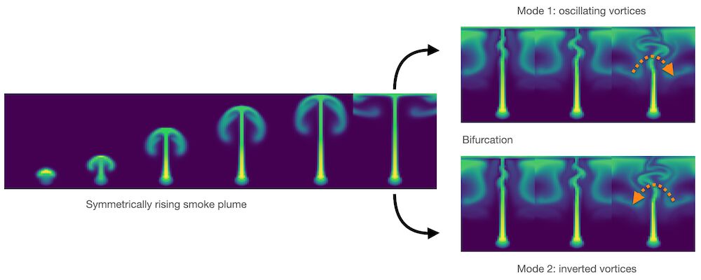
Fig. 3 A bifurcation in a buoyancy-driven fluid flow: the “smoke” shown in green color starts rising in a perfectly straight manner, but tiny numerical inaccuracies grow over time to lead to an instability with vortices alternating to one side (top-right), or in the opposite direction (bottom-right).

Next steps

For each of the following notebooks, there’s a “next steps” section like the one below which contains recommendations about where to start modifying the code. After all, the whole point of these notebooks is to have readily executable programs as a basis for own experiments. The data set and NN sizes of the examples are often quite small to reduce the runtime of the notebooks, but they’re nonetheless good starting points for potentially complex and large projects.

For the simple DP example above:

• This notebook is intentionally using a very simple setup. You can change the training setup or network architectures to improve the solutions. E.g., provide more samples around zero to improve the solution near the origin.

• Or try extending the setup to a 2D case, i.e. a paraboloid. Given the function \(\mathcal P:(y_1,y_2)\to y_1^2+y_2^2\), find an inverse function \(f\) such that \(\mathcal P(f(x)) = x\) for all \(x\) in \([0,1]\).

• If you want to experiment without installing anything, you can also [run this notebook in colab].