Half-Inverse Gradients#
The scale-invariant physics updates (SIPs) of the previous chapters illustrated the importance of inverting the direction of the update step (in addition to making use of higher order terms). We’ll now turn to an alternative for achieving the inversion, the so-called Half-Inverse Gradients (HIGs) [SHT22]. They come with their own set of pros and cons, and thus provide an interesting alternative for computing improved update steps for physics-based deep learning tasks.
Unlike the SIPs, they do not require an analytical inverse solver. The HIGs jointly invert the neural network part as well as the physical model. As a drawback, they require an SVD for a large Jacobian matrix.
Preview: HIGs versus SIPs (and versus Adam)
More specifically the HIGs:
do not require an analytical inverse solver (in contrast to SIPs),
and they jointly invert the neural network part as well as the physical model.
As a drawback, HIGs:
require an SVD for a large Jacobian matrix,
and are based on first-order information (similar to regular gradients).
Howver, in contrast to regular gradients, they use the full Jacobian matrix. So as we’ll see below, they typically outperform regular GD and Adam significantly.
Derivation#
As mentioned during the derivation of inverse simulator updates in (34), the update for regular Newton steps uses the inverse Hessian matrix. If we rewrite its update for the case of an \(L^2\) loss, we arrive at the Gauss-Newton (GN) method:
For a full-rank Jacobian \(\partial y / \partial \theta\), the transposed Jacobian cancels out, and the equation simplifies to
This looks much simpler, but still leaves us with a Jacobian matrix to invert. This Jacobian is typically non-square, and has small singular values which cause problems during inversion. Naively applying methods like Gauss-Newton can quickly explode. However, as we’re dealing with cases where we have a physics solver in the training loop, the small singular values are often relevant for the physics. Hence, we don’t want to just discard these parts of the learning signal, but rather preserve as many of them as possible.
This motivates the HIG update, which employs a partial and truncated inversion of the form
where the square-root for \(^{-1/2}\) is computed via an SVD, and denotes the half-inverse. I.e., for a matrix \(A\), we compute its half-inverse via a singular value decomposition as \(A^{-1/2} = V \Lambda^{-1/2} U^T\), where \(\Lambda\) contains the singular values. During this step we can also take care of numerical noise in the form of small singular values. All entries of \(\Lambda\) smaller than a threshold \(\tau\) are set to zero.
Note
Truncation versus Clamping: It might seem attractive at first to clamp singular values to a small value \(\tau\), instead of discarding them by setting them to zero. However, the singular vectors corresponding to these small singular values are exactly the ones which are potentially unreliable. A small \(\tau\) yields a large contribution during the inversion, and thus these singular vectors would cause problems when clamping. Hence, it’s a much better idea to discard their content by setting their singular values to zero.
The use of a partial inversion via \(^{-1/2}\) instead of a full inversion with \(^{-1}\) helps preventing that small eigenvalues lead to overly large contributions in the update step. This is inspired by Adam, which normalizes the search direction via \(J/(\sqrt(diag(J^{T}J)))\) instead of inverting it via \(J/(J^{T}J)\), with \(J\) being the diagonal of the Jacobian matrix. For Adam, this compromise is necessary due to the rough approximation via the diagonal. For HIGs, we use the full Jacobian, and hence can do a proper inversion. Nonetheless, as outlined in the original paper [SHT22], the half-inversion regularizes the inverse and provides substantial improvements for the learning, while reducing the chance of gradient explosions.
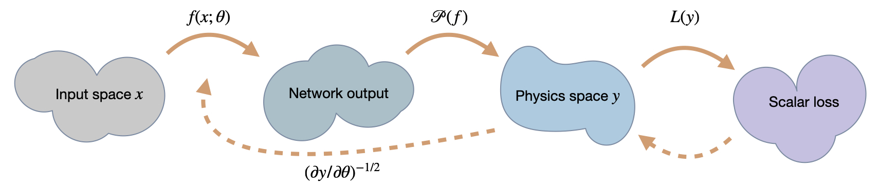
Fig. 55 A visual overview of the different spaces involved in HIG training. Most importantly, it makes use of the joint, inverse Jacobian for neural network and physics.#
Constructing the Jacobian#
The formulation above hides one important aspect of HIGs: the search direction we compute not only jointly takes into account the scaling of neural network and physics, but can also incorporate information from all the samples in a mini-batch. This has the advantage of finding the optimal direction (in an \(L^2\) sense) to minimize the loss, instead of averaging directions as done with GD or Adam.
To achieve, this, the Jacobian matrix for \(\partial y / \partial \theta\) is concatenated from the individual Jacobians of each sample in a mini-batch. Let \(x_i,y_i\) denote input and output of sample \(i\) in a mini-batch, respectively, then the final Jacobian is constructed via all the \(\frac{\partial y_i}{\partial \theta}\big\vert_{x_i}\) as
The notation with \(\big\vert_{x_i}\) also makes clear that all parts of the Jacobian are evaluated with the corresponding input states. In contrast to regular optimizations, where larger batches typically don’t pay off too much due to the averaging effect, the HIGs have a stronger dependence on the batch size. They often profit from larger mini-batch sizes.
To summarize, compute the HIG update requires evaluating the individual Jacobians of a batch, doing an SVD of the combined Jacobian, truncating and half-inverting the singular values, and computing the update direction by re-assembling the half-inverted Jacobian matrix.

Properties Illustrated via a Toy Example#
This is a good time to illustrate the properties mentioned in the previous paragraphs with a real example. As learning target, we’ll consider a simple two-dimensional setting with the function
and a scaled loss function
Here \(y_1\) and \(y_2\) denote the first, and second component of \(y\) (in contrast to the subscript \(i\) used for the entries of a mini-batch above). Note that the scaling via \(\lambda\) is intentionally only applied to the second component in the loss. This mimics an uneven scaling of the two components as commonly encountered in physical simulation settings, the amount of which can be chosen via \(\lambda\).
We’ll use a small neural network with a single hidden layer consisting of 7 neurons with tanh() activations and the objective to learn \(\hat{y}\).
Well-conditioned#
Let’s first look at the well-conditioned case with \(\lambda=1\). In the following image, we’ll compare Adam as the most popular GD-representative, Gauss-Newton (GN) as “classical” method, and the HIGs. These methods are evaluated w.r.t. three aspects: naturally, it’s interesting to see how the loss evolves. In addition, we’ll consider the distribution of neuron activations from the resulting neural network states (more on that below). Finally, it’s also interesting to observe how the optimization influences the resulting target states (in \(y\) space) produced by the neural network. Note that the \(y\)-space graph below shows only a single, but fairly representative, \(x,y\) pair. The other two show quantities from a larger set of validation inputs.
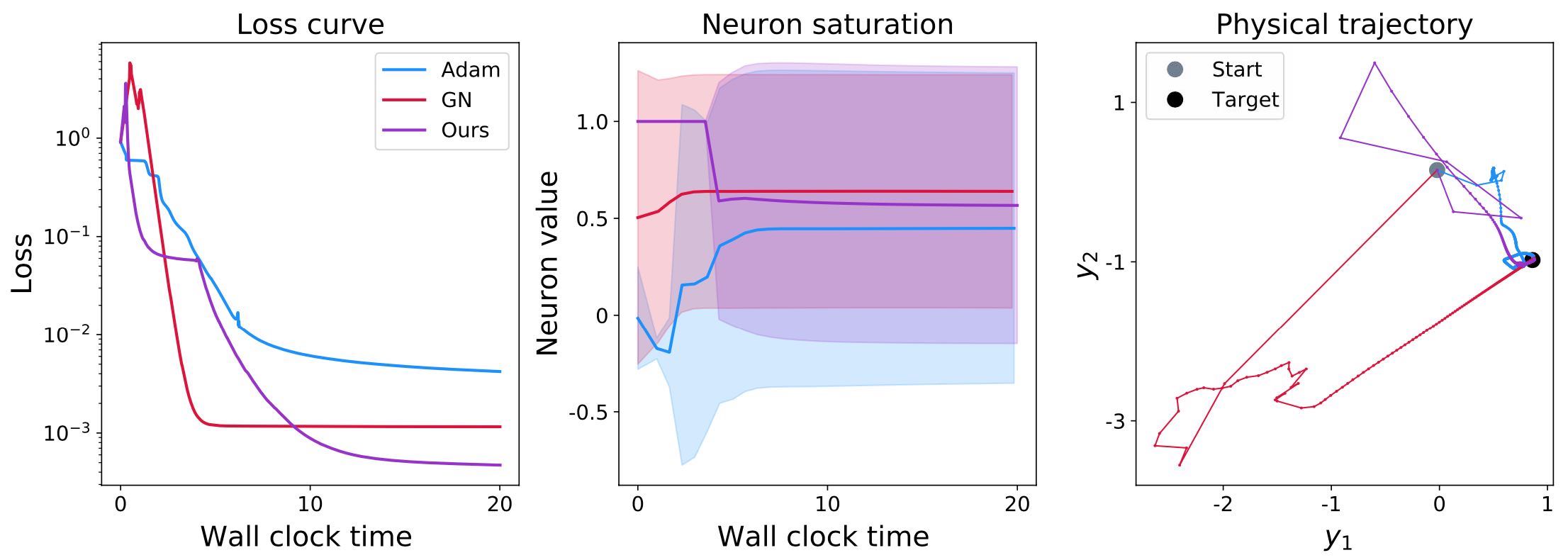
Fig. 56 The example problem for a well-conditioned case. Comparing Adam, GN, and HIGs.#
As seen here, all three methods fare okay on all fronts for the well conditioned case: the loss decreases to around \(10^{-2}\) and \(10^{-3}\).
In addition, the neuron activations, which are shown in terms of mean and standard deviation, all show a broad range of values (as indicated by the solid-shaded regions representing the standard deviation). This means that the neurons of all three networks produce a wide range of values. While it’s difficult to interpret specific values here, it’s a good sign that different values are produced by different inputs. If this was not the case, i.e., different inputs producing constant values (despite the obviously different targets in \(\hat{y}\)), this would be a very bad sign. This is typically caused by fully saturated neurons whose state was “destroyed” by an overly large update step. But for this well-conditioned toy example, this saturation is not showing up.
Finally, the third graph on the right shows the evolution in terms of a single input-output pair. The starting point from the initial network state is shown in light gray, while the ground truth target \(\hat{y}\) is shown as a black dot. Most importantly, all three methods reach the black dot in the end. For this simple example, it’s not overly impressive to see this. However, it’s still interesting that both GN and HIG exhibit large jumps in the initial stages of the learning process (the first few segments leaving the gray dot). This is caused by the fairly bad initial state, and the inversion, which leads to significant changes of the NN state and its outputs. In contrast, the momentum terms of Adam reduce this jumpiness: the initial jumps in the light blue line are smaller than those of the other two.
Overall, the behavior of all three methods is largely in line with what we’d expect: while the loss surely could go down more, and some of the steps in \(y\) seem to momentarily do in the wrong direction, all three methods cope quite well with this case. Not surprisingly, this picture will change when making things harder with a more ill-conditioned Jacobian resulting from a small \(\lambda\).
Ill-conditioned#
Now we can consider a less well-conditioned case with \(\lambda=0.01\). The conditioning could be much worse in real-world PDE solvers, but interestingly, this factor of \(1/100\) is sufficient to illustrate the problems that arise in practice. Here are the same 3 graphs for the ill-conditioned case:
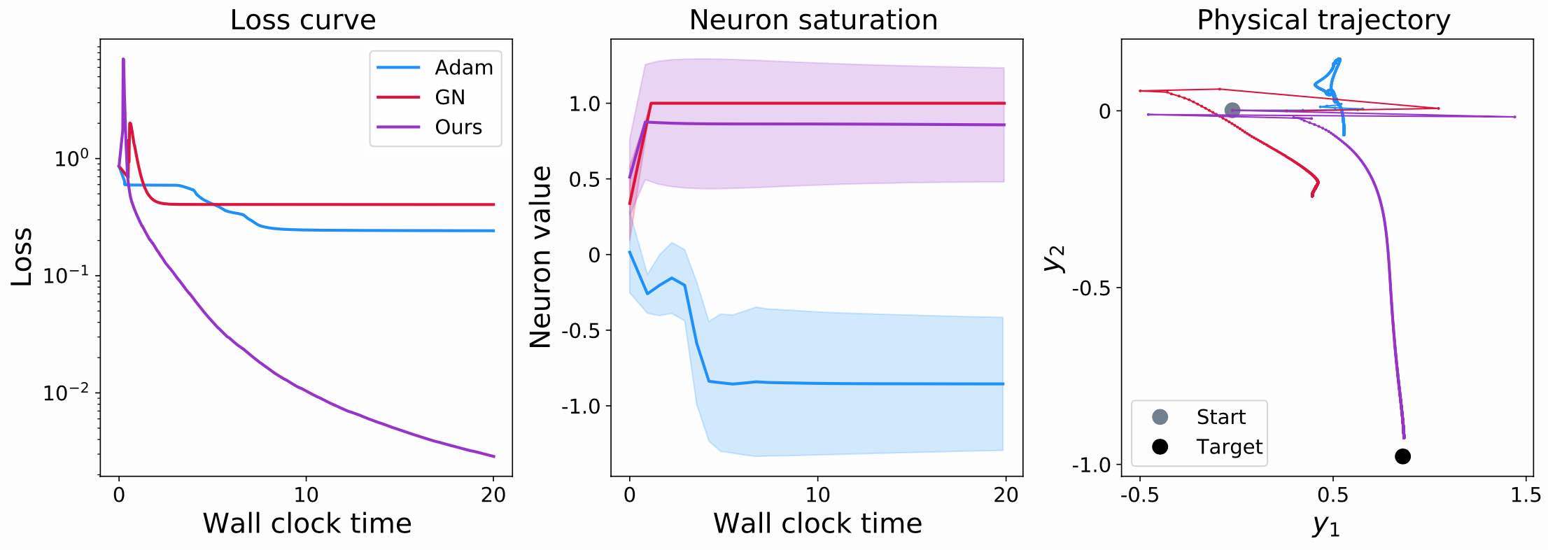
Fig. 57 The example problem for an ill-conditioned case. Comparing Adam, GN, and HIGs.#
The loss curves now show a different behavior: both Adam and GN do not manage to decrease the loss beyond a level of around 0.2 (compared to the 0.01 and better from before). Adam has significant problems with the bad scaling of the \(y^2\) component, and fails to properly converge. For GN, the complete inversion of the Jacobians causes gradient explosions, which destroy the positive effects of the inversion. Even worse, they cause the neural network to effectively get stuck.
This becomes even clearer in the middle graph, showing the activations statistics. The red curve of GN very quickly saturates at 1, without showing any variance. Hence, all neurons have saturated, and do not produce meaningful signals anymore. This not only means that the target function isn’t approximated well, it also means that future gradients will effectively be zero, and these neurons are lost to all future learning iterations. Hence, this is a highly undesirable case that we want to avoid in practice. It’s also worth pointing out that this doesn’t always happen for GN. However, it regularly happens, e.g. when individual samples in a batch lead to vectors in the Jacobian that are linearly dependent (or very close to it), and thus makes GN a sub-optimal choice.
The third graph on the right side of figure Fig. 57 shows the resulting behavior in terms of the outputs. As already indicated by the loss values, both Adam and GN do not reach the target (the black dot). Interestingly, it’s also apparent that both have much more problems along the \(y^2\) direction, which we used to cause the bad conditioning: they both make some progress along the x-axis of the graph (\(y^1\)), but don’t move much towards the \(y^2\) target value. This is illustrating the discussions above: GN gets stuck due to its saturated neurons, while Adam struggles to undo the scaling of \(y^2\).
Summary of Half-Inverse Gradients#
Note that for all examples so far, we’ve improved upon the differentiable physics (DP) training from the previous chapters. I.e., we’ve focused on combinations of neural networks and PDE solving operators. The latter need to be differentiable for training with regular GD, as well as for HIG-based training.
In contrast, for training with SIPs (from Scale Invariant Physics Training), we even needed to provide a full inverse solver. As shown there, this has advantages, but differentiates SIPs from DP and HIGs. Thus, the HIGs share more similarities with, e.g., Reducing Numerical Errors with Neural Operators and Solving Inverse Problems with NNs, than with the example Learning to Invert Heat Conduction with Scale-invariant Updates.
This is a good time to give a specific code example of how to train physical NNs with HIGs: we’ll look at a classic case, a system of coupled oscillators.