Integrating DP into NN Training#
We’ll now target integrations of differentiable physics (DP) setups into NNs. When using DP approaches for learning applications, there is a lot of flexibility w.r.t. the combination of DP and NN building blocks. As some of the differences are subtle, the following section will go into more detail. We’ll especially focus on solvers that repeat the PDE and NN evaluations multiple times, e.g., to compute multiple states of the physical system over time. In classical numerics, this would be called an iterative time stepping method, while in the context of AI, it’s an autoregressive method.
Hint: Correction vs Prediction
The problems that are best tackled with DP approaches are very fundamental. The combination of a imperfect physical model and an improvement term classically goes under many different names: closure problems in fluid dynamics and turbulence, homogenization or coarse-graining in material science, while it’s called parametrization in climate and weather.
In the following, we’ll generically denote all these tasks containing NN+solver as correction task, in contrast to pure prediction tasks for cases where no solver is involved at inference time.
To re-cap, here’s the previous figure about combining NNs and DP operators. In the figure these operators look like a loss term: they typically don’t have weights, and only provide a gradient that influences the optimization of the NN weights:
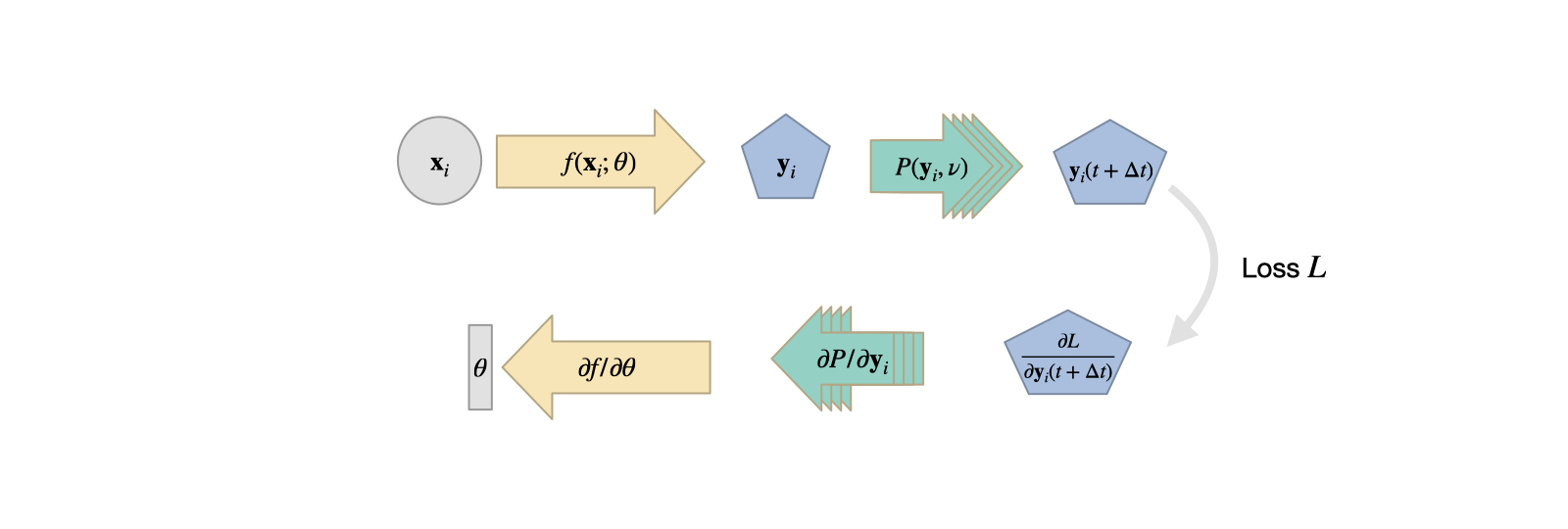
Fig. 18 The DP approach as described in the previous chapters. A network produces an input to a PDE solver \(\mathcal P\), which provides a gradient for training during the backpropagation step.#
This setup can be seen as the network receiving information about how it’s output influences the outcome of the PDE solver. I.e., the gradient will provide information how to produce an NN output that minimizes the loss. Similar to the previously described Physical Loss Terms, this can, e.g., mean upholding a conservation law or generally a PDE-based constraint over time.
Switching the order#
However, with DP, there’s no real reason to be limited to this setup. E.g., we could imagine a swap of the NN and DP components, giving the following structure:
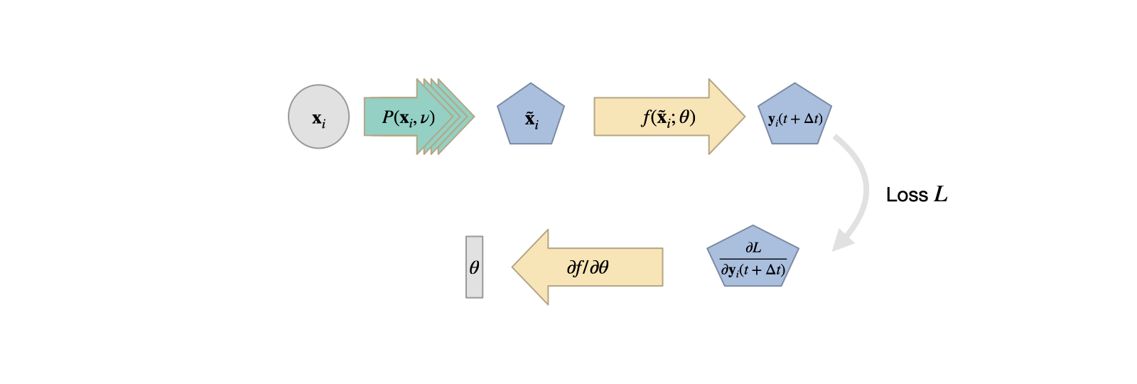
Fig. 19 A PDE solver produces an output which is processed by an NN.#
In this case the PDE solver essentially represents an on-the-fly data generator. That’s not necessarily always useful: this setup could be replaced by a pre-computation of the same inputs, as the PDE solver is not influenced by the NN. Hence, there’s no backpropagation through \(\mathcal P\), and it could be replaced by a simple “loading” function. On the other hand, evaluating the PDE solver at training time with a randomized sampling of input parameters can lead to an excellent sampling of the data distribution of the input. If we have realistic ranges for how the inputs vary, this can improve the NN training. If implemented correctly, the solver can also alleviate the need to store and load large amounts of data, and instead produce them more quickly at training time, e.g., directly on a GPU. Recent methods explore this direction in the context of Active Learning.
However, this version does not leverage the gradient information from a differentiable solver, which is why the following variant is more interesting.
Recurrent evaluation#
A combination that makes particular sense is to unroll the iterations of a time stepping process of a simulator, and let the state of a system be influenced by an NN. (In general, there’s no combination of NN layers and DP operators that is forbidden (as long as their dimensions are compatible).)
In the case of unrolling, we compute a (potentially very long) sequence of PDE solver steps in the forward pass. In-between these solver steps, an NN modifies the state of our system, which is then used to compute the next PDE solver step. During the backpropagation pass, we move backwards through all of these steps to evaluate contributions to the loss function (it can be evaluated in one or more places anywhere in the execution chain), and to backprop the gradient information through the DP and NN operators. This unrollment of solver iterations essentially gives feedback to the NN about how it’s “actions” influence the state of the physical system and resulting loss. Here’s a visual overview of this form of combination:
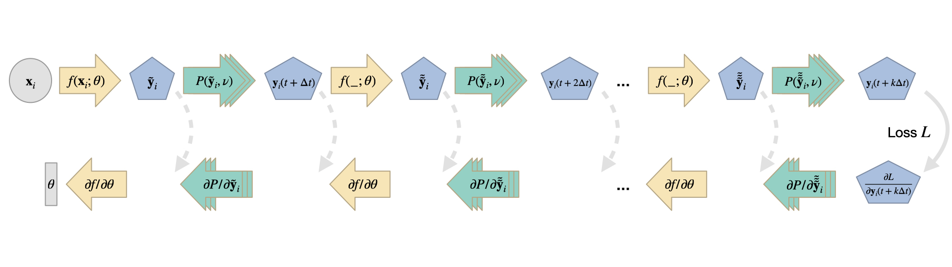
Fig. 20 Time stepping with interleaved DP and NN operations for \(k\) solver iterations. The dashed gray arrows indicate optional intermediate evaluations of loss terms (similar to the solid gray arrow for the last step \(k\)), and intermediate outputs of the NN are indicated with a tilde.#
Due to the iterative nature of this process, errors will start out very small, and then (for modes with eigenvalues larger than one in the Jacobian) slowly increase exponentially over the course of iterations. Hence they are extremely difficult to detect in a single evaluation, e.g., with a simpler supervised training setup. Rather, it is crucial to provide feedback to the NN at training time how the errors evolve over course of the iterations. Additionally, a pre-computation of the states is not possible for such iterative cases, as the iterations depend on the state of the NN. Naturally, the NN state is unknown before training time and changes while being trained. This is the classic ML problem of data shift. Hence, a DP-based training is crucial in these recurrent settings to provide the NN with gradients about how its current state influences the solver iterations, and correspondingly, how the weights should be changed to better achieve the learning objectives.
DP setups with many time steps can be difficult to train: the gradients need to backpropagate through the full chain of PDE solver evaluations and NN evaluations. Typically, each of them represents a non-linear and complex function. Hence for larger numbers of steps, the vanishing and exploding gradient problem can make training difficult. Some practical considerations for alleviating this will follow int Reducing Numerical Errors with Neural Operators.

Composition of NN and solver#
One question that we have ignored so far is how the merge the output of the NN into the iterative solving process. In the images above, it looks like the NN \(f\) produces a full state of the physical system, that is used as input to \(\mathcal P\). That means for a state \(x(t+j \Delta t)\) at step \(j\), the NN yields an intermediate state \(\tilde x(t+j \Delta t) = f(x(t+j \Delta t); \theta)\), with which the solver produces the new state for the following step: \(x(t+ (j+1) \Delta t) = \mathcal P(\tilde x(t+j \Delta t))\).
While this approach is possible, it is not necessarily the best in all cases. Especially if the NN should produce only a correction of the current state, we can reuse parts of the current state. This avoids allocating resources of the NN in the form of parts of \(\theta\) to infer the parts that are already correct. Along the lines of skip connections in a U-Net and the residuals of a ResNet, in these cases it’s better to use an operator \(\circ\) that merges \(x\) and \(\tilde x\), i.e. \(x(t+ (j+1) \Delta t) = \mathcal P(x(t+j \Delta t) \circ \tilde x(t+j \Delta t))\). In the simplest case, we can define \(\circ\) to be an addition, in which case \(\tilde x\) represents an additive correction of \(x\). In short, we evaluate \(\mathcal P(x + \tilde x)\) to compute the next state. Here the network only needs to update the parts of \(x\) that don’t yet satisfy the learning objective.
In general, we can use any differentiable operator for \(\circ\), it could be a multiplication or an integration scheme. Similar to the loss function, this choice is problem dependent, but an addition is usually a good starting point.
In equation form#
Next, we’ll formalize the descriptions of the previous paragraphs. Specifically, we’ll answer the question: what does the resulting update step for \(\theta\) look like in terms of Jacobians? Given mini batches with an index \(i\), a loss function \(L\), we’ll use \(k\) to denote the total number of steps that are unrolled for an iteration. To shorten the notation, \(x_{i,j} = x_i(t + j \Delta t) \) denotes a state \(x\) of batch \(i\) at time step \(j\). With this notation we can write the gradient of the network weights as:
This doesn’t look too intuitive on first sight, but this expression has a fairly simple structure: the first sum for \(i\) simply accumulates all entries of a mini batch. Then we have an outer summation over \(m\) (the brackets) that accounts for all time steps from \(1\) to \(k\). For each \(m\), we’ll trace the chain from the final state \(k\) back to each \(m\) by multiplying up all Jacobians along the way (with index \(n\), in parentheses). Each step along the way is made up of a Jacobian w.r.t. \(x\) for each time step, which in turn depends on the correction from the NN \(\tilde x\) (not written out).
At each last step \(m\) for the neural network we “branch-off” and determine the change in terms of the network output \(\tilde x\) and its weights \(\theta\) at the \(m\)’th time step. All these contributions for different \(m\) are added up to give a final update \(\Delta \theta\) that is used in the optimizer of our training process.
It’s important to keep in mind that for large \(m\), the recurrently applied Jacobians of \(\mathcal P\) and \(f\) strongly influence the contributions of later time steps, and hence it is critical to stabilize the training to prevent exploding gradients, in particular. This is a topic we will re-visit several time later on.
In terms of implementation, all deep learning frameworks will re-use the overlapping parts that repeat for different \(m\). This is automatically handled in the backprop evaluation, and in practice, the sum will be evaluated from large to small m, such that we can “forget” the later steps when moving towards small \(m\). So the backprop step definitely increases the computational cost, but it’s usually on a similar order as the forward pass, provided that we have suitable operators to compute the derivatives of \(\mathcal P\).
Backpropagation through solver steps#
Now that we have all this machinery set up, a good question to ask is: “How much does training with a differentiable physics simulator really improve things? Couldn’t we simply unroll a supervised setup, along the lines of standard recurrent training, without using a differentiable solver?” Or to pose it differently, how much do we really gain by backpropagating through multiple steps of the solver?
In short, quite a lot! The next paragraphs show an evaluation for a turbulent mixing layer from List et al. [LCT22], case to illustrate this difference. Before going into details, it worth noting that this comparison uses a differentiable second-order semi-implicit flow solver with a set of custom turbulence loss terms. So it’s not a toy problem, but shows the influence of differentiability for a complex, real-world case.
The nice thing about this case is that we can evaluate it in terms of established statistic measurements for turbulence cases, and quantify the differences in this way. The energy spectrum of the flow is typically a starting point here, but we’ll skip it and refer to the original paper [LCT22], and rather focus on two metrics that are more informative. The graphs below show the Reynolds stresses and the turbulence kinetic energy (TKE), both in terms of resolved quantities for a cross section in the flow. The reference solution is shown with orange dots.
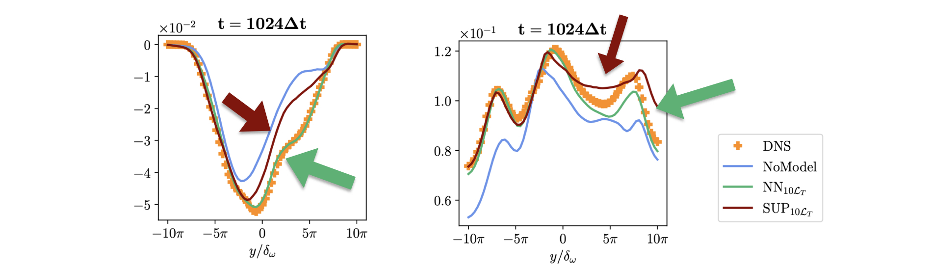
Fig. 21 Quantified evaluation with turbulence metrics: Reynolds stresses (L) and TKE (R). The red curve of the training without a differentiable solver deviates more strongly from the ground truth (orange dots) than the training with DP (green).#
Especially in the regions indicated by the colored arrows, the red curve of the “unrolled supervised” training deviates more strongly from the reference solution. Both measurements are taken after 1024 time steps of simulation using the fluid solver in conjunction with a trained NN. Hence, both solutions are quite stable, and fare significantly better than the unmodified output of the solver, which is shown in blue in the graphs.
The differences are also very obvious visually, when qualitatively comparing visualizations of the vorticity fields:
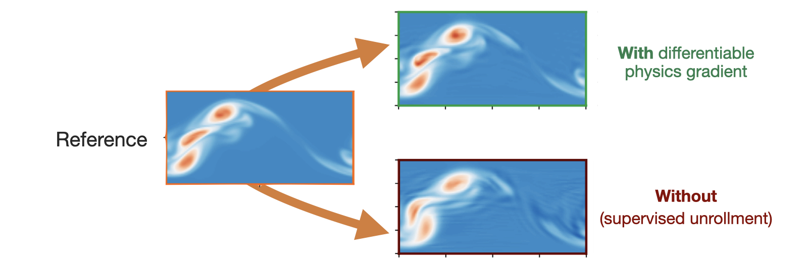
Fig. 22 Qualitative , visual comparison in terms of vorticity. The training with a differentiable physics solver (top) results in structures that better preserve those of the reference solution obtained via a direct numerical simulation.#
Both versions, with and without solver gradients strongly benefit from unrollment, for 10 steps in this comparison. However, the supervised variant without DP cannot use longer-term information about the effects of the NN at training time, and hence its capabilities are limited. The version trained with the differentiable solver receives feedback for the whole course of the 10 unrolled steps, and in this way can infer corrections the give an improved accuracy for the resulting, NN-powered solver.
As an outlook, this case also highlights the practical advantages of incorporating NNs into solvers: we can measure how long a regular simulation would take to achieve a certain accuracy in terms of turbulence statistics. For this case it would require more than 14x longer than the solver with the NN [LCT22]. While this is just a first data point, it’s good to see that, once a network is trained, real-world improvements in terms of performance can be achieved more or less out-of-the-box.
Alternatives: noise#
Other works have proposed perturbing the inputs and the iterations at training time with noise [SGGP+20], somewhat similar to regularizers like dropout. This can help to prevent overfitting to the training states, and in this way can help to stabilize training iterative solvers.
However, the noise is very different in nature. It is typically undirected, and hence not as accurate as training with the actual evolutions of simulations. So noise can be a good starting point for training setups that tend to overfit. However, if possible, it is preferable to incorporate the actual solver in the training loop via a DP approach to give the network feedback about the time evolution of the system.
With the current state of affairs, generative modeling approaches (denoising diffusion or flow matching) or provide a better founded approach for incorporating noise. We’ll look into this topic in more detail in Unconditional Stability.
Complex examples#
The following sections will give code examples of more complex cases to show what can be achieved via differentiable physics training.
First, we’ll show a scenario that employs deep learning to represent the errors of numerical simulations, following Um et al. [UBH+20]. This is a very fundamental task, and requires the learned model to closely interact with a numerical solver. Hence, it’s a prime example of situations where it’s crucial to bring the numerical solver into the deep learning loop.
Next, we’ll show how to let NNs solve tough inverse problems, namely the long-term control of a Navier-Stokes simulation, following Holl et al. [HKT19]. This task requires long term planning, and hence needs two networks, one to predict the evolution, and another one to act to reach the desired goal. (Later on, in Controlling Burgers’ Equation with Reinforcement Learning we will compare this approach to another DL variant using reinforcement learning.)
Both cases require quite a bit more resources than the previous examples, so you can expect these notebooks to run longer (and it’s a good idea to use check-pointing when working with these examples).